This article is an end-to-end walkthrough of FlexiBuild Studio to build a supervised machine-learning pipeline, using a banking use case as an example.
Watch the walkthrough video:
Introduction
The AI & Analytics Engine provides two fundamental ways for users to build their ML solutions and use them:
FlexiBuild Studio provides you with an easy-to-use no-code tool to define, compose, and run custom ML pipelines to suit various business use cases.
In this article, a banking use case is used to walk you through the process of building and using an ML pipeline.
The binary classification banking use case
Consider a scenario where your role is a data analyst/scientist in a banking institution, and your objective is to use data to optimize the loan approval process.
The main challenge is to distinguish between loan applicants who are likely to repay their loans on time, and those who are prone to default or delay their payments, by building a model that learns from historical transactions of loan applicants and their final outcomes.
This is a binary classification problem, where the features are derived from the loan applications, the customer demographics, and their historical transactions, with the target variable being the loan status (no problem or debt).
Datasets
📂The Czech bank dataset was used for this guide. Why not download the datasets and generate your own predictions?
The input data for this use case consists of three tables:
Loans dataset: This table contains information about loan applications, such as loan ID, customer ID, loan amount, loan duration, and loan status. The loan status is a categorical column with four possible values:
-
A (finished, no problem),
-
B (finished, debt),
-
C (running, no problem), and
-
D (running, debt).
The loan status column will be transformed into a binary column with two values: no problem and debt, which will be used as the target column for the classification problem.
Clients dataset: This table contains customer records containing the following attributes: gender, date of birth, and location.
Transactions dataset: This table of historical records of customer transactions. Each record contains the customer ID, transaction date, transaction amount, transaction type, and balance.
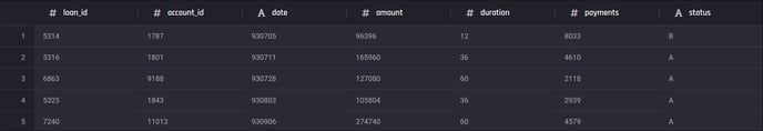 Preview of the loans table
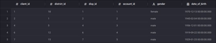 Preview of the clients table
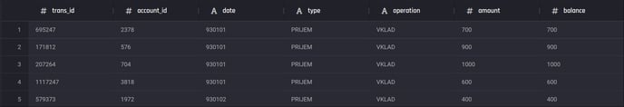 Preview of the transactions table
Getting started with the App Builder
The first step is to log in to the Engine and ensure that you are in the right project in which you want to create the app. From the options shown to build your app, choose Regression or classification under FlexiBuild Studio, since our use case is a classification task:
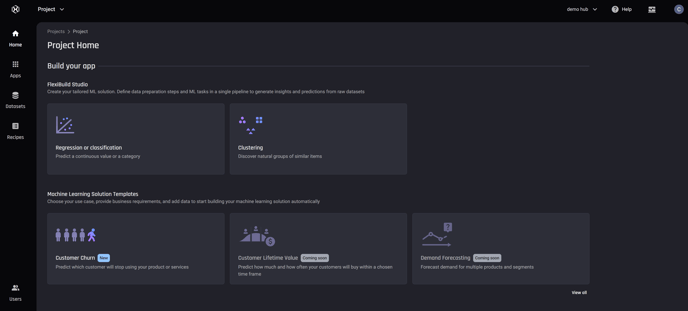 Project Homepage, select app builder Regression or classification under FlexiBuild Studio
Once you confirm the app name, you are taken to the App builder view. It contains the following steps.
-
Prepare data
-
Define what to predict (the target column and the problem type)
-
Select the features and
-
Build models
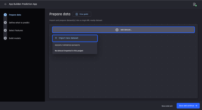
Step 1: Prepare data
In the first step, the goal is to add the three datasets relevant to the use case and generate a single dataset containing the feature columns and the target column. This single dataset is called an ML-ready dataset.
🎓 An ML-ready dataset is required to build ML model. For more information, read what is a machine learning-ready dataset
To do this, you can either add existing datasets from the same project that you had previously imported or you can import a new one. Since there are no existing datasets, proceed with the Import option.
 App builder pipeline, import new data into app
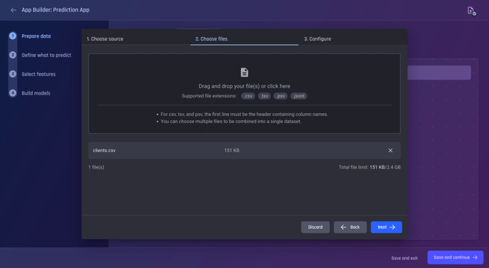
Under the import options choose Local file upload and then choose the file you want to upload and proceed. Choose the clients dataset for upload.
 Choose the clients.csv file
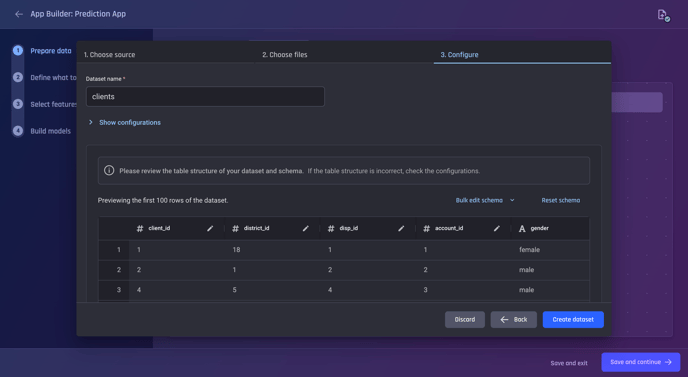
After choosing your file, you can proceed to the next step where you can see the preview and the schema.
 Preview and Configure Step
The schema that the Engine has inferred looks satisfactory, especially since it has correctly detected the type of date_of_birth as datetime and all other columns except gender as numeric.
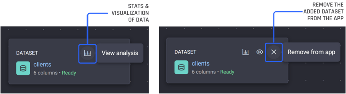
Upon confirming the creation of the dataset, you are taken back to the app builder pipeline view where you can see the added dataset.
You can examine the column stats and visualizations with the View Analysis icon or remove the dataset from the app (but keep it in the project) with the cross icon.
 Dataset Options
Proceed by adding the remaining two datasets: loans.csv and transactions.csv. so you now have the three datasets in your app.
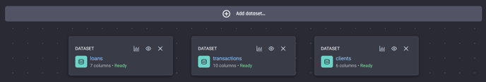 App builder pipeline with all three datasets added
Preparing the ML-ready dataset
The next step is to prepare datasets. The goal is to have a single dataset at the end that contains all the information about the loans, stats from the customers' transaction history, and their demographic information in a single tabular-form dataset, so we have an ML-ready dataset to proceed with.
You can use the View guide link in the header to learn more. Keep an eye out for such guides to familiarize yourself with the steps needed to be taken within the Engine.
Continuing with the use case, first prepare the loans and transactions datasets.
Preparing the transactions dataset
To prepare a dataset, first, click on it and choose the option Prepare data.
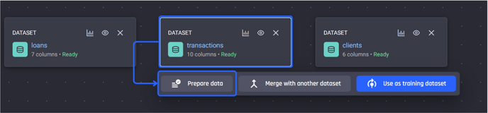 Transactions dataset selected, click on Prepare data
There are three options:
-
Create a new recipe
-
Copy and modify an existing recipe
-
Apply an existing recipe as-is without modification
🎓 For more information, read What is a recipe
Choose the first option, Create a new recipe and name your recipe “Prepare transactions”.
You are then taken to the recipe builder where you can start adding actions to prepare your data. Within the recipe editor, you can see a preview of the dataset after the added actions have been applied.
None have been added yet. So you're just seeing the preview of the original data. To add actions to your recipe use the right-side panel and select Add action.
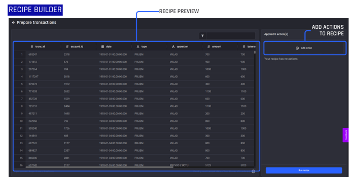 The recipe builder, with actions added on the right and a preview pane visible to the left so you can review actions performed against the dataset
💡Tip: The actions needed to prepare datasets differ from dataset to dataset and use case to use case, so can not be prescribed for you in this guide for your own real-life use case. It is decided by you based on your understanding of the dataset, the domain, and the business problem.
For the transactions dataset, you need a translation of the non-English (Czech language) labels in the type column into English-language labels.
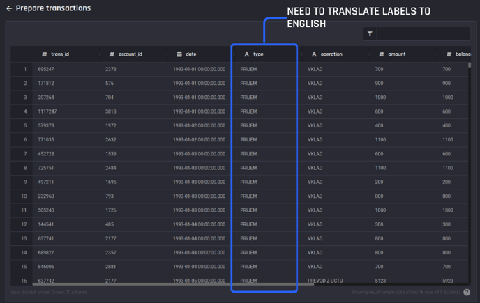 Recipe builder, column type requires labels translated to English via adding a mapping action
To do this, select “Add action” and search for “Map to text” using the search bar under “All actions”. You then add the action and configure it properly.
-
Select the input column, here it is the type column.
-
Apply the following translations:
-
PRIJEM -> credit
-
VYDAJ -> withdrawal
-
VYBER -> withdrawal_cash
-
-
Once the configuration is completed, add the action.
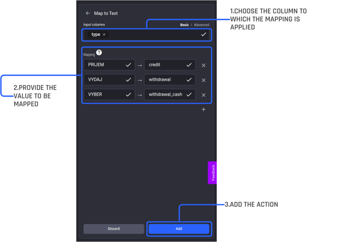 Recipe builder, configuring the action “Map to Text”
You can see the action is added to the recipe and that the preview has been updated to include the action applied to the dataset as you can now see the translated labels for column type.
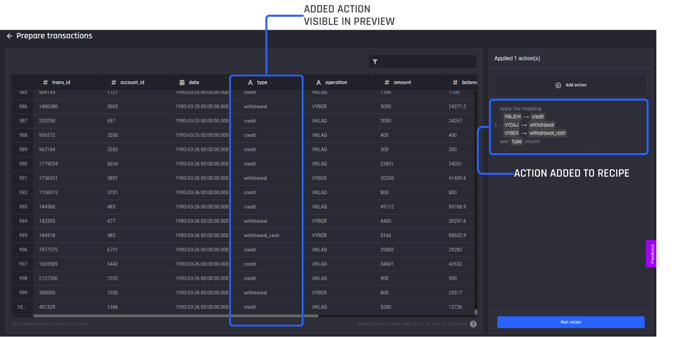 Values for type column have been updated as per the added action
Once an action is added to a recipe, if you need to change it, you have the Edit and Delete options available.
Having ensured we have added the actions we want to the recipe, finish it by clicking Run recipe and providing a name for the output dataset. After the output name is confirmed, you can see the recipe and the output dataset being generated in the Prepare data stage of the app pipeline builder.
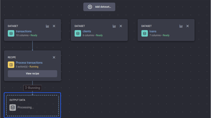 A recipe in “Running” status with the output dataset yet to be generated
You don't need to wait for the processing, you can proceed to prepare the next dataset which is loans.
Preparing the loans dataset
Create a new recipe for loans. Apply the following actions to the recipe.
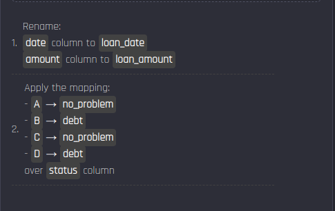 The recipe for the loans dataset
Finish the recipe by issuing Run recipe.
After both recipes finish running, you can see both have produced prepared datasets as outputs.
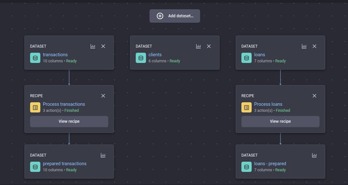 The recipes for preparing the transactions and loans have finished running and the prepared datasets are available
Aggregating and joining to generate the final dataset, the ML-ready dataset
Next, you want to generate additional features to predict the loan status, this process is called feature engineering.
💡Feature engineering refers to the process of using domain knowledge to select and transform the most relevant variables in your raw data. The goal of feature engineering and selection is to improve the performance of ML algorithms.
To do so, you need to aggregate stats of transactions over the past up to and until the loan application dates.
In turn, you should also join the transactions dataset with the loans dataset and filter out transactions that happened later than the loan date, before computing the aggregation, to avoid data leakage from the future into the present.
You can do that by selecting the prepared transactions dataset and then selecting the Merge with another dataset option this time.
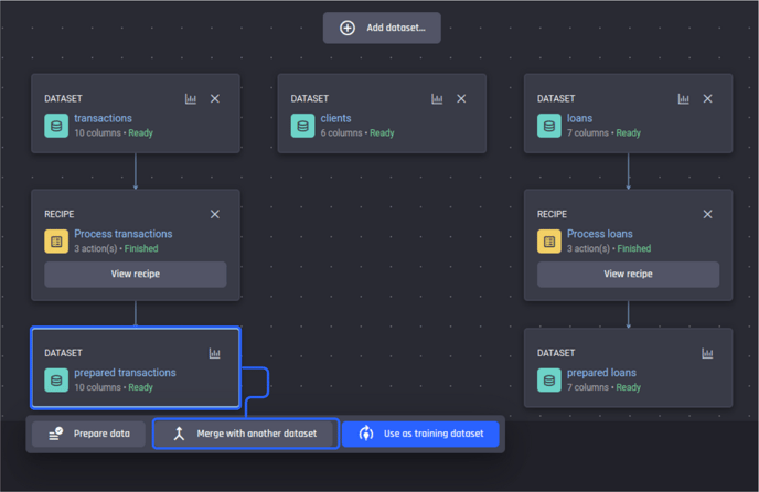 Select the output dataset from the “process transactions” recipe, then join it with another dataset
This process also creates a recipe, but conveniently adds the action to merge the two datasets on your behalf.
You are shown different ways to “merge with a dataset”. Joins such as left join, outer join, and inner join, lookup values from another dataset, and aggregate-lookup. Use the “join” option.
Select the dataset to join with the “prepared transactions” dataset, which is the prepared loans dataset, then click Create recipe.
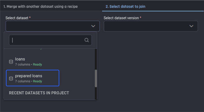 Selecting the dataset to merge with
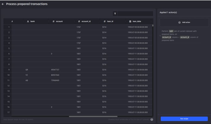
You will be taken to the recipe builder view with the join action open, where you can modify and confirm the join parameters inferred by the Engine.
Configure the join type as a “right” join, since you are only interested in the transactions from accounts that have a loan.
From the loans dataset, you can keep all columns except for the account_id, as the transaction dataset already has an account id.
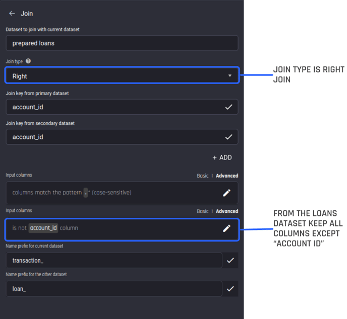 A selected merging action is added to a new editable recipe. We can customize the action further
Save changes to add the action, you can see columns added from the prepared loans dataset as well.
 Result of the join action. You can see the columns added from the loans dataset
Next, you want to remove the entries where the transaction date is past the loan date, so that you don't leak data from the future into the past.
To do this, choose the “filter rows” action within the “All actions” catalog, and enter the formula date < loan_date to keep only the rows satisfying this criterion.
 The (boolean) criterion we want to filter by: Use only the transaction history that happened before the loan agreement date
Then for each loan, compute the following aggregate stats:
-
Number of transactions of each type
-
Minimum, maximum, mean, median, and standard deviation of:
-
amounts for each transaction type
-
interval between transactions of each type
-
-
Days since the last transaction of each type
To facilitate finding the average interval between transactions of each type, you first want to compute the lag function of the date column, partitioned by account_id and type, ordered by the date column.
This can be accomplished with the “Shift rows…” action within the "All actions" catalog.
Name the output column produced by this action as previous_date_of_same_transaction_type
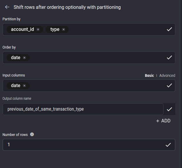 Configuring the “Shift rows” action: We want to partition by both the account_id and type columns to compute the lagged date that contains the date of the previous transaction of the same type from the same customer as the current transaction
Add this action, and then compute the number of days elapsed between date and previous_date_of_same_transaction_type using the “compute time elapsed” action, naming the output as days_since_last_transaction_of_same_type.
Note that you need to specify the optional time unit” parameter as days instead of leaving it to be the default setting of seconds.
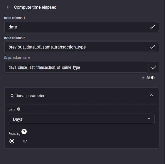 Configuring the “Compute time elapsed” action: We want to subtract the date of the previous transaction of the same type from the date of the current transaction, to get the intervals in days between successive transactions of the same type
Then, to compute multiple stats for each transaction type, make use of the “Reshape dataset into a pivot table” action, specifying account_id for the group-by column, type for the pivot column, and credit, withdrawal, and withdrawal_cash for the pivot values. Then add multiple aggregates as follows:
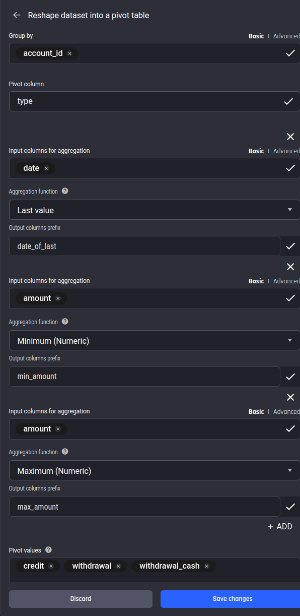 Using the “Pivot” action to compute aggregate features: We pivot by the transaction’s type to get stats of the amount and interval in days columns under the specified transaction types (pivot values) separately
After this, add a few more actions.
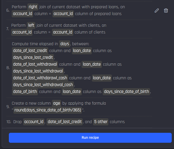 Completing the final recipe with the required actions: Getting the features from the loans dataset back, then getting features from the clients dataset, computing recency and age features
The reasoning behind these actions
After adding the pivot action to compute aggregates by transaction type, the columns from the “loans” dataset were lost, you can get them back by joining again using the same join keys.
You then join with the “clients” data to get the demographic features date_of_birth, age and district_id.
Then, you extract more features from the datetime columns:
-
Days since last transaction of each type at loan-application day: using the “Compute time elapsed” action
-
Age of the person: using the “Compute time elapsed” action, followed by division by 365 to convert days to years
As a final step, you drop all columns of DateTime type (as you have already extracted features from them) and the intermediate column storing the age in days instead of years.
You can now run this recipe to produce the output.
 Output dataset of the recipe joining and aggregating from three sources
You need one more important feature from the transactions dataset: The minimum balance at the time of loan application.
To get this feature, you start again from the prepared transactions dataset. You will be joining with both the prepared loans dataset and the dataset output by the latest recipe we worked on.
Here is a summary of the recipe:
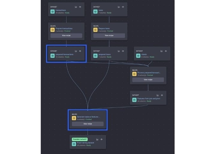 Recipe to generate the minimum balance feature and the input dataset it is created from
 Recipe to generate the balance aggregation features
You do a right join with the prepared loans dataset and filter out transactions whose dates are later than the loan application date.
Then compute the minimum of the balance column grouped by the account_id column. Then join with the features that you generated before, using the account_id column as the key.
Selecting the training dataset
You have now produced your ML-ready training dataset. To proceed, select the final dataset and set it to Use as a training dataset. Then click Save and continue to proceed to the next step, Define what to predict.

Step 2: Selecting the target column and problem type
Select the target column. Here, it is the column named status (the loan status).
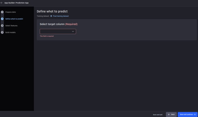 The target column needs to be specified
Once the column is chosen, the Engine automatically selects Binary classification with debt as the positive label and disables Regression, as you are predicting two classes with labels debt and no problem.
You can also configure the train/test split. For this use case, leave it as the default of 80% train (and 20% test).
🎓 For more information about train/test splits read What is the train test split for classification and regression apps
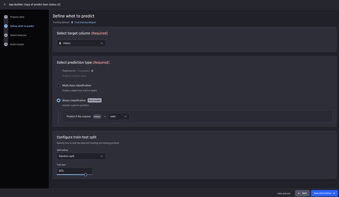 For the specified target column, the prediction type and the train/test split configuration can be chosen
Select Save and continue to proceed to the next step 3 Feature selection.
Step 3: Selecting features
Here, you can either let the Engine:
-
Automatically select the best set of features such that the top most features with a total estimated importance reaches a desired percentage threshold
-
Manually select the features with the feature-importance estimates.
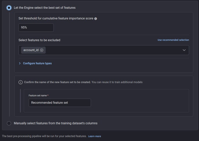 Selecting features: Automatic and manual options
If confident, you have the option to manually select any or all of them. When manually selecting the features you also have the following options to utilize to make a more informed decision.
-
Use analysis column to understand the feature statistics
-
Let the Engine estimate the feature importance and use them. Here again, you can specify which columns must not be considered as candidate features.
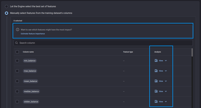 Option to estimate feature importance and look into analysis of the feature
 Feature selection, the Engine is computing feature importance estimates
Once the estimation is done, you can sort features by importance and select the topmost features that reach a certain total percentage threshold.
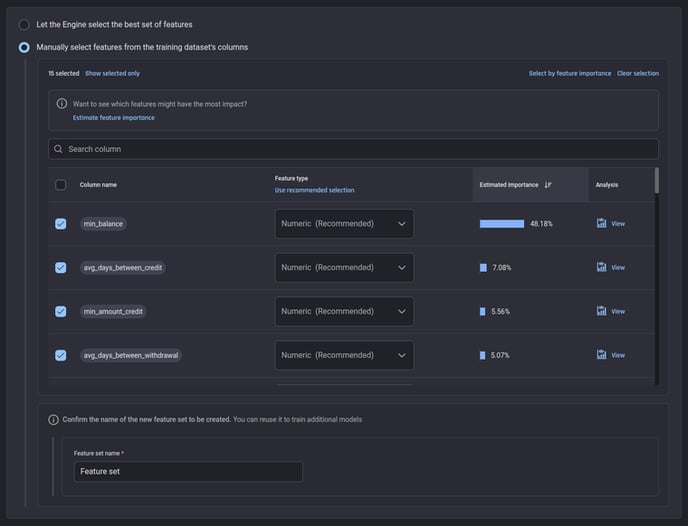 Features ordered by estimated importance: Available when the Engine finishes analyzing data
In both automatic and manual options, the feature types are automatically recommended by the Engine, however you have the option to change the feature types if required. In this case, all features are Numeric; with no nominal (categorical) or descriptive (text) features.
Once you are satisfied with the selected features, you can name the feature set to reuse the same set of features later if required.
💡The Engine uses Generative AI to make this step easy for you:
-
It automatically suggests the columns to be estimated from consideration, both for the automatic and manual options. Here, the Engine recommends account_id to be removed from consideration.
-
It automatically suggests the correct feature type based on the analysis of the column and inferring the meaning of a column from the context of the dataset.
Step 4: Selecting algorithms to train ML models
In the final step of the app pipeline builder, you need to specify how the Engine should train the ML models.
You can:
-
Let the Engine choose the best algorithms and train them based on estimates that satisfy certain desired criteria, or:
-
You can manually choose them.
For this use case, opt for the former, letting the Engine choose 3 algorithms with an estimated prediction quality of at least 60% and an estimated training time of less than 2 hours.
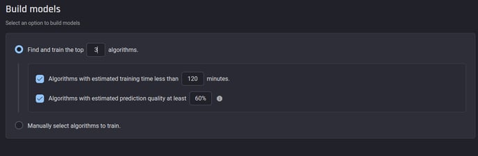 Letting the Engine select algorithms. You can specify selection criteria to optimize the outcome
Select Save and continue, so that the app starts processing datasets and training models.
Finishing the process with the App summary page
You will be taken to the App summary page, showing the progress status of various steps.
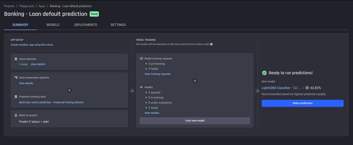
When the app finishes processing and models are trained, the top model’s performance will appear on the right side, along with the prediction quality.
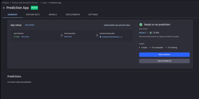 Summary page of an app in “Ready” state. We can train more models, or make predictions when one or more models have finished training
Understanding your model
Head to the Model tab, from there you can select any model by clicking the name of the model. This will take you to the Model summary page.
Model Insights – Evaluation and Explainability
You can see 72.58% prediction quality, which is great given that the ratio of debt to no_problem cases is very small in the dataset.
Upon clicking the model name from this section, you can see details about the model, and what you can do with it.
Select View details” for the performance card.
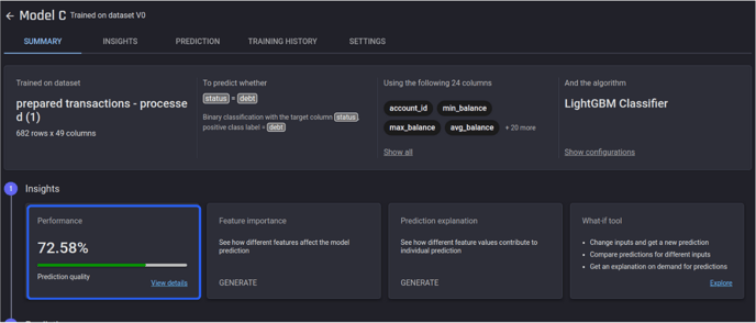 The model details page
Here you can see the detailed evaluation report, including the metrics and charts. For binary classification problems such as this, you can change the threshold and see how the metrics and the confusion matrix change with it.
🎓 To learn more about model evaluation metrics read Which metrics are used to evaluate a binary classification model's performance?
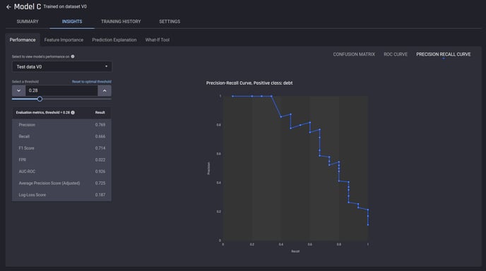 Evaluation metrics and charts for the trained model
In the Feature Importance tab, you can generate feature importances, so that you understand which features impact the model most.
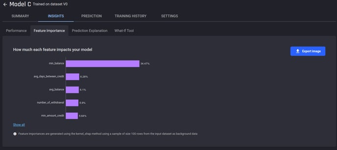 The generated feature importance scores for our model
This will also generate the Prediction Explanation for a sample of the predictions generated on the test portion, available in the next tab.
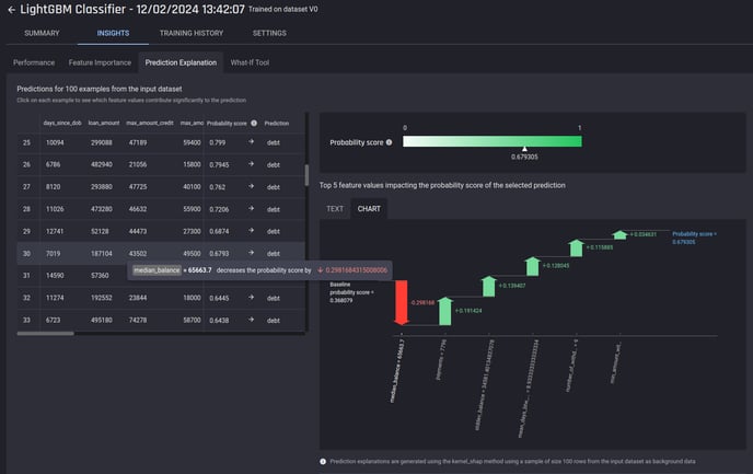 Sample prediction explanations generated for our model
Making predictions with trained models
If you are satisfied with the model’s performance and the insights that explain how the model makes predictions.
The next step is to make predictions whenever you have new data, there are two ways to make predictions:
-
One-off prediction
-
Scheduled periodic predictions
First select Make predictions from the App summary page, and choose to make either one-off or scheduled predictions.
 Making predictions: Access from the summary page of the app
Either option will take you to the prediction pipeline page, where you can see the recommended model selected already, you have the option to use a different model if desired.
In the next step, you can visualize the prediction pipeline builder. There are placeholders to add the input datasets first, with the links to the corresponding datasets used in training under each.
Here, you can either add a dataset directly or configure a data source (such as a database connection) to ingest the latest data from a table on a periodic basis, if using the “Schedule periodic predictions” option.
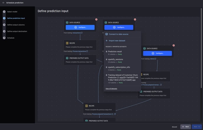 The prediction pipeline to be configured: Placeholders for input datasets and recipes are shown, following the same structure created in Step 1 of the app builder
Once an input dataset is added, the corresponding recipe(s) will be populated as its child node(s), if one or more recipes were applied at the time of training to the corresponding training dataset.
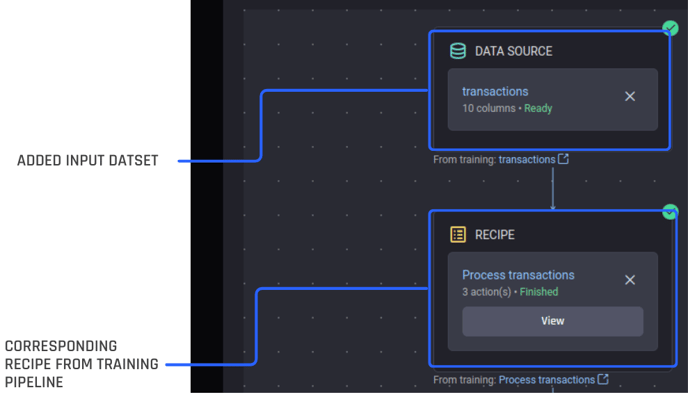 Recipes are populated once an input dataset is added
You can also remove these recipes and add modifiable copies of the original recipe if you wish to make changes to the training recipe. This might be necessary for example to remove recipe actions added at the time of building the app to generate/modify the target column.
 Remove a recipe and replace it with another one or create a new one to run during the prediction
After adding all the input datasets and the recipes, and all recipes and model inputs are validated, the configuration will be shown as “completed” and you can proceed to the next step.
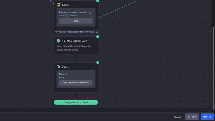 Completed prediction-pipeline configuration: Prediction dataset and model
The prediction will appear as a tabular dataset with these additional columns, along with the features used to make predictions (output of the final recipe before the model).
In the next step, you can configure the names of these prediction output columns. Here, since the use case is binary classification, we can also choose the threshold applied to the probability to get the binary label. Here is an example configuration:
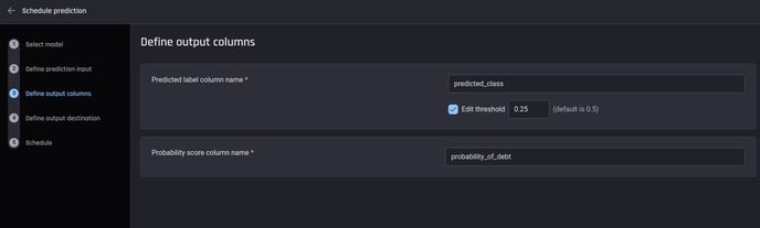 Configuring the names of the prediction-output columns
After this, you can optionally define output destinations for the predictions.
The same prediction can be sent to different output destinations simultaneously. This can be either to a project within the organization with the current projeect being the default or a database table connection.
This step is optional; predictions will still be available under the app for download/export later even if no output destinations are defined at this point. If using scheduled predictions, in the next step you can configure when predictions should be run.
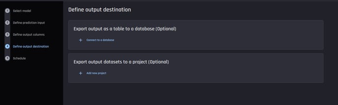 Optionally, predictions generated can be exported into different destinations
Once all these steps are completed, either:
-
A prediction run is immediately started, if making a one-off prediction, or;
-
A prediction run will start at the scheduled date/time on a periodic basis.
Once a prediction run starts, it takes a few minutes to generate the final predictions, depending on the size of the datasets and the complexity of the data-preparation pipeline.
You can predictions on the app summary page with the status indicators.
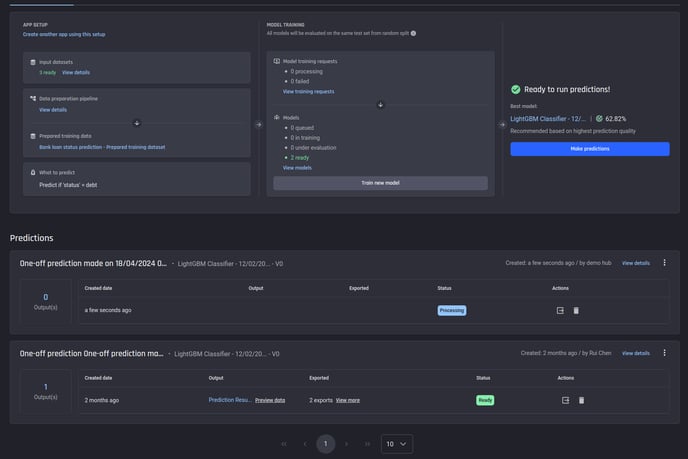 Predictions that have run will appear in the summary page of the app
Once predictions are ready, you can use the the icons under Actions consume the predictions several ways.
-
Preview the predictions
-
Export the predictions via
-
Downloading them as a file
-
Exporting them into a project within the Engine
-
Exporting them to a external database table
-
%20or%20exported.png?width=688&height=120&name=Results%20can%20be%20previewed%2c%20downloaded%20(as%20file)%20or%20exported.png) Prediction run finished: Results can be previewed, downloaded (as a file) or exported
Prediction run finished: Results can be previewed, downloaded (as a file) or exported
Select Preview details to view a preview of the dataset. Here you can see that the last two columns contain the prediction outputs i.e., the predicted label for the given threshold and the probability score produced by the model.
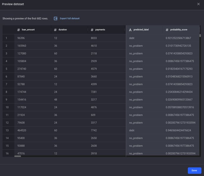 Prediction output preview
Conclusion
You have built an application and generated predictions on new data for a loan-status prediction use case in the banking industry. The following is a summary of the steps taken:
-
Prepared an ML-ready training dataset.
-
Defined the target column for prediction, chose features, and applied the best algorithms to train your models.
-
Re-use the recipes used to generate the training dataset at prediction time, to transform new data coming in the original schema into an ML-ready prediction dataset.
-
Specified additional configurations such as choosing between different types of problems (multi-class vs. binary classification) and the positive class label