.png?width=800&name=Blog%20Images%20(83).png)


.png?width=800&name=Blog%20Images%20(84).png)
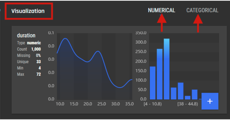
.png?width=800&name=Blog%20Images%20(85).png) Although the number of examples for good is slightly more than bad, it is not a severely imbalanced dataset and hence we can proceed with building our model. If for example, we had 990 examples for good and only 10 examples for bad, then that would have meant that our dataset is highly skewed and we should balance the classes.
Although the number of examples for good is slightly more than bad, it is not a severely imbalanced dataset and hence we can proceed with building our model. If for example, we had 990 examples for good and only 10 examples for bad, then that would have meant that our dataset is highly skewed and we should balance the classes..png?width=800&name=Blog%20Images%20(86).png)
.png?width=1000&name=Blog%20Images%20(87).png)
.png?width=1000&name=Blog%20Images%20(88).png)
.png?width=800&name=Blog%20Images%20(89).png)

.png?width=800&name=Blog%20Images%20(90).png)
.png?width=800&name=Blog%20Images%20(91).png)
.png?width=800&name=Blog%20Images%20(92).png)
.png?width=800&name=Blog%20Images%20(93).png)
.png?width=800&name=Blog%20Images%20(94).png)
.png?width=800&name=Blog%20Images%20(95).png)
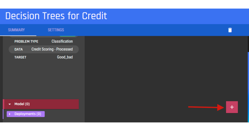
.png?width=800&name=Blog%20Images%20(96).png) And we are done with the Python implementation. Now let’s do the same on the AI & Analytics Engine
And we are done with the Python implementation. Now let’s do the same on the AI & Analytics Engine .png?width=800&name=Blog%20Images%20(97).png)
.png?width=800&name=Blog%20Images%20(98).png)
.png?width=800&name=Blog%20Images%20(99).png)
.png?width=800&name=Blog%20Images%20(100).png)


ML for small businesses
How to Affordably Upscale Your Small Business with Machine Learning
How do you upscale your current product offering affordably with ml, for small businesses? There are a few basic problems a startup will encounter.